Physics COMBINATION OF CAPACITORS, ENERGY STORED IN A CAPACITOR FOR CBSE-NCERT-6

Topic covered

`color{blue}{star}` COMBINATION OF CAPACITORS
`color{blue}{star}` ENERGY STORED IN A CAPACITOR
`color{blue}{star}` VAN DE GRAAFF GENERATOR

COMBINATION OF CAPACITORS

`color{blue} ✍️` We can combine several capacitors of capacitance `C_1, C_2,…, C_n` to obtain a system with some effective capacitance `C`.

`color{blue} ✍️` The effective capacitance depends on the way the individual capacitors are combined. Two simple possibilities are discussed below.

`color{purple}bbul("Capacitors in series")`

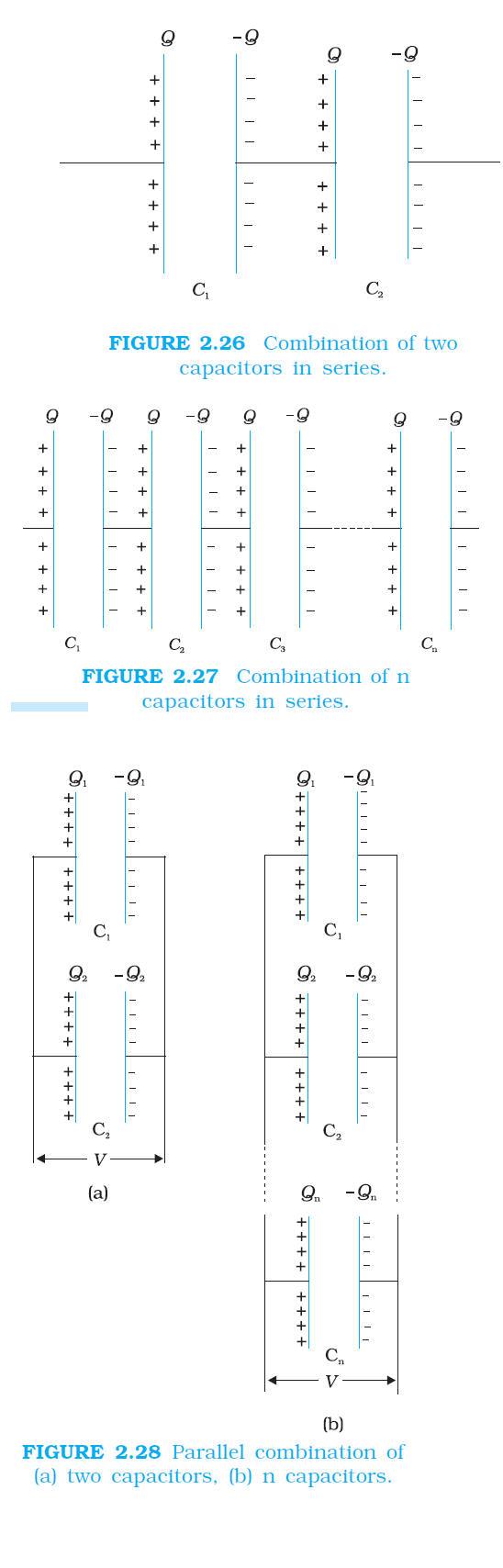
`color{blue} ✍️` Figure 2.26 shows capacitors `C_1` and `C_2` combined in series.

`color{blue} ✍️` The left plate of `C_1` and the right plate of `C_2` are connected to two terminals of a battery and have charges `Q` and `–Q,` respectively. It then follows that the right plate of `C_1` has charge `–Q` and the left plate of `C_2` has charge `Q.`

`color{blue} ✍️` If this was not so, the net charge on each capacitor would not be zero. This would result in an electric field in the conductor connecting `C_1` and `C_2`.

`color{blue} ✍️` Charge would flow until the net charge on both `C_1` and `C_2` is zero and there is no electric field in the conductor connecting `C_1` and `C_2`.

`color{blue} ✍️`Thus, in the series combination, charges on the two plates `(±Q)` are the same on each capacitor. The total potential drop V across the combination is the sum of the potential drops `V_1` and `V_2` across `color{purple}(C_1` and `C_2)`, respectively.


`color{purple}(V= V_1 + V_2 = Q/(C_1) + Q/(C_2))` .....................2.55

`color{purple}(i.e V/Q = 1/(C_1) + 1/(C_2))` .......................2.56

`color{blue} ✍️` Now we can regard the combination as an effective capacitor with charge Q and potential difference V. The effective capacitance of the combination is

`color{purple}(C= Q/V)` ...................2.57

We compare Eq. (2.57) with Eq. (2.56), and obtain

`color{purple}(1/C= 1/(C_1) + 1/(C_2))` ........................... 2.58


`color{blue} ✍️` The proof clearly goes through for any number of capacitors arranged in a similar way. Equation (2.55), for n capacitors arranged in series, generalises to

`color{purple}(V = V_1 +V_2 + .. + V_n = Q/(C_1) + Q/(C_2) +.....+ Q/(C_n))` ............... 2.59


`color{blue} ✍️` Following the same steps as for the case of two capacitors, we get the general formula for effective capacitance of a series combination of n capacitors:

`color{purple}(1/C = 1/(C_1) + 1/(C_2) + 1/(C_3) + 1/(C_n))`

............................ 2.60


`color{blue} bbul{"Capacitors in parallel "}`

`color{blue} ✍️` Figure 2.28 (a) shows two capacitors arranged in parallel. In this case, the same potential difference is applied across both the capacitors. But the plate charges `(±Q_1)` on capacitor 1 and the plate charges `(±Q_2)` on the capacitor 2 are not necessarily the same:


`color{purple}(Q_1 = C_1V, Q_2 = C_2V)` .......................2.61

`color{blue} ✍️` The equivalent capacitor is one with charge

`color{purple}(Q = Q_1 + Q_2)` ........................ 2.62

and potential difference `V`.

`color{purple}(Q = CV = C_1V + C_2V)` .......................2.63

`color{blue} ✍️` The effective capacitance C is, from Eq. (2.63),

`color{purple}(C = C_1 + C_2)` .................2.64

`color{blue} ✍️` The general formula for effective capacitance C for parallel combination of n capacitors [Fig. 2.28 (b)] follows similarly


`color{purple}(Q = Q_1 + Q_2 + ... + Q_n_)` ..................2.65

`color{purple}(i.e., CV = C_1V + C_2V + ... C_nV)` ...............2.66
which gives

`color{purple}(C = C_1 + C_2 + ... C_n)`

............................2.67


Q 3174880756

A network of four 10 μF capacitors is connected to a 500 V supply, as shown in Fig. 2.29. Determine (a) the equivalent capacitance of the network and (b) the charge on each capacitor. (Note, the charge on a capacitor is the charge on the plate with higher potential, equal and opposite to the charge on the plate with lower potential.)
Class 12 Chapter example 9
Solution:

(a) In the given network, `C_1, C_2` and `C_3` are connected in series. The effective capacitance C′ of these three capacitors is given by

`1/C = 1/C_1+1/C_2 +1/C_3`
For `C_1 = C_2 = C_3 = 10 μF, C′ = (10/3) μF.` The network has C′ and `C_4`
connected in parallel. Thus, the equivalent capacitance C of the
network is

`C = C′ + C_4 = (10/3 +10) mu F = 13.3 muF`
b) Clearly, from the figure, the charge on each of the capacitors, `C_1,`
`C_2` and `C_3` is the same, say Q. Let the charge on C4 be Q′. Now, since
the potential difference across AB is `Q//C_1`, across BC is `Q//C_2`, across

CD is `Q//C3` , we have

`Q/(C_1)+ Q/(C_2) + Q/(C_3) = 500V`

Also, `Q′//C_4 = 500 V.`

This gives for the given value of the capacitances,

`Q = 500 V xx 10/3 muF = 1.7 xx 10^(-3) C` and
`Q = 500V xx 10 mu F = 5.0 xx 10^(-3) C`

ENERGY STORED IN A CAPACITOR

`color{blue} ✍️` A capacitor, as we have seen above, is a system of two conductors with charge `Q` and `–Q. `

`color{blue} ✍️` To determine the energy stored in this configuration, consider initially two uncharged conductors `1` and `2`. Imagine next a process of transferring charge from conductor `2` to conductor 1 bit by bit, so that at the end, conductor `1` gets charge `Q`.

`color{blue} ✍️` By charge conservation, conductor `2` has charge `–Q` at the end (Fig 2.30 ).

`color{blue} ✍️` In transferring positive charge from conductor `2` to conductor `1`, work will be done externally, since at any stage conductor `1` is at a higher potential than conductor `2`.

`color{blue} ✍️` To calculate the total work done, we first calculate the work done in a small step involving transfer of an infinitesimal (i.e., vanishingly small) amount of charge. Consider the intermediate situation when the conductors 1 and 2 have charges Q′ and –Q′ respectively.

`color{blue} ✍️` At this stage, the potential difference `V′` between conductors `1` to 2 is `Q′//C,` where `C` is the capacitance of the system. Next imagine that a small charge `δ Q′` is transferred from conductor `2` to `1`. Work done in this step `(δ W′ )`, resulting in charge Q′ on conductor 1 increasing to `color{purple}(Q′+ δ Q′)`, is given by

`color{purple}(δW = V′δQ' = (Q')/C δQ')` ....................... 2.68

`color{blue} ✍️` Since `δ Q′` can be made as small as we like, Eq. (2.68) can be written as

`color{purple}(δW = 1/(2C) [(Q' + δQ')^2-Q'^2])` ..................2.69

`color{blue} ✍️` Equations (2.68) and (2.69) are identical because the term of second order in δ Q′, i.e., `δ Q′ 2//2C`, is negligible, since `δ Q′` is arbitrarily small. The total work done (W) is the sum of the small work `(δ W)` over the very large number of steps involved in building the charge Q′ from zero to Q.

`color{purple}(W= underset("sum over all steps")sum ( deltaW)`

`color{purple}(W = underset("sum over all steps")sum 1/(2C) [(Q' δQ')^2-Q'^2])` ................... 2.70

`color{purple}(= 1/(2C) [(deltaQ'^2 -o')+{(2deltaQ')^2 - deltaQ'^2} + {(3deltaQ'^2)-(2deltaQ')^2}+.....+{Q^2-(Q_deltaQ)^2})` ......2.71

`color{purple}(= 1/(2C) {Q^2-0] = (Q^2)/(2C))` ...................2.72

The same result can be obtained directly from Eq. (2.68) by integration

`color{green}(W = int_(0)^(Q) 1/CdeltaQ' = 1/C (Q'^2)/2 |_(0)^(Q) = (Q^2)/(2C))`


`color{blue} ✍️` This is not surprising since integration is nothing but summation of a large number of small terms.
We can write the final result, Eq. (2.72) in different ways

`color{purple}(W = (Q^2)/(2C) = 1/2 CV^2 = 1/2 QV)` ......................2.73

`color{blue} ✍️` Since electrostatic force is conservative, this work is stored in the form of potential energy of the system.

`color{blue} ✍️` For the same reason, the final result for potential energy [Eq. (2.73)] is independent of the manner in which the charge configuration of the capacitor is built up.

`color{blue} ✍️` When the capacitor discharges, this stored-up energy is released. It is possible to view the potential energy of the capacitor as ‘stored’ in the electric field between the plates. To see this, consider for simplicity, a parallel plate capacitor [of area A(of each plate) and separation d between the plates]. Energy stored in the capacitor

`color{purple}(1/2 (Q^2)/C = (Asigma)^2/2 xx d/(epsilon_0A))` ........................ 2.74

`\color{green} ✍️` The surface charge density `σ` is related to the electric field `E` between the plates,

`color{purple}(E= (sigma)/(epsilon_0))` .................2.74

From Eqs. (2.74) and (2.75) , we get Energy stored in the capacitor

`color{purple}(U = (1/2)ε_0 E^2 × Ad)` .......................2.76

`color{blue} ✍️` Note that Ad is the volume of the region between the plates (where electric field alone exists). If we define energy density as energy stored per unit volume of space, Eq (2.76) shows that Energy density of electric field,

`color{purple}(u =(1/2)ε_0E^2)` ..........................2.77

`color{blue} ✍️` Though we derived Eq. (2.77) for the case of a parallel plate capacitor, the result on energy density of an electric field is, in fact, very general and holds true for electric field due to any configuration of charges.
Q 3114880759

A 900 pF capacitor is charged by 100 V battery [Fig. 2.31(a)]. How much electrostatic energy is stored by the capacitor? (b) The capacitor is disconnected from the battery and connected to another 900 pF capacitor [Fig. 2.31(b)]. What is the electrostatic energy stored by the system?
Class 12 Chapter example 10
Solution:

(a) The charge on the capacitor is
`Q = CV = 900 × 10^(–12) F × 100 V = 9 × 10^(–8) C`
The energy stored by the capacitor is
`= (1//2) CV^2 = (1//2) QV`
`= (1/2) × 9 × 10^(–8)C × 100 V = 4.5 × 10^(–6) J`
(b) In the steady situation, the two capacitors have their positive plates at the same potential, and their negative plates at the same potential. Let the common potential difference be `V′.` The charge on each capacitor is then `Q′ = CV`′. By charge conservation, `Q′ = Q//2.` This implies `V′ = V//2.`The total energy of the system is

`= 2xx1/2 Q 'V = 1/4 QV = 2.25 xx 10^(-6) J`
Thus in going from (a) to (b), though no charge is lost; the final energy is only half the initial energy. Where has the remaining energy gone? There is a transient period before the system settles to the situation (b). During this period, a transient current flows from the first capacitor to the second. Energy is lost during this time in the form of heat and electromagnetic radiation.

VAN DE GRAAFF GENERATOR

`color{blue} ✍️` This is a machine that can build up high voltages of the order of a few million volts.

`color{blue} ✍️` The resulting large electric fields are used to accelerate charged particles (electrons, protons, ions) to high energies needed for experiments to probe the small scale structure of matter. The principle underlying the machine is as follows.

`color{blue} ✍️` Suppose we have a large spherical conducting shell of radius `R`, on which we place a charge `Q`. This charge spreads itself uniformly all over the sphere. As we have seen in Section 1.14, the field outside the sphere is just that of a point charge Q at the centre; while the field inside the sphere vanishes.

`color{blue} ✍️` So the potential outside is that of a point charge; and inside it is constant, namely the value at the radius `R`. We thus have: Potential inside conducting spherical shell of radius `R` carrying charge `Q =` constant

`color{purple}(= 1/(4piepsilon_0) Q/(R))` ............................2.78

`color{blue} ✍️` Now, as shown in Fig. 2.32, let us suppose that in some way we introduce a small sphere of radius `r`, carrying some charge `q`, into the large one, and place it at the centre.

`color{blue} ✍️` The potential due to this new charge clearly has the following values at the radii indicated: Potential due to small sphere of radius `r` carrying charge `q`

`color{purple}(= 1/(4piepsilon_0) q/r` at surface of small sphere

`color{purple}(= 1/(4piepsilon_0) q/R` at large shell of radius `R`. ....................2.79


Taking both charges `q` and `Q` into account we have for the total potential `V` and the potential difference the values

`color{purple}(V (R)= 1/(4piepsilon_0)(Q/R+q/R))`

`color{purple}(V (r)= 1/(4piepsilon_0)(Q/R+q/r))`

`color{purple}(V (r)= q/(4piepsilon_0)(1/r-1/R))`

.........................2.80

`color{blue} ✍️` Assume now that `q` is positive. We see that, independent of the amount of charge `Q` that may have accumulated on the larger sphere and even if it is positive, the inner sphere is always at a higher potential: the difference `V(r )–V(R)` is positive.

`color{blue} ✍️` The potential due to `Q` is constant upto radius `R` and so cancels out in the difference , This means that if we now connect the smaller and larger sphere by a wire, the charge `q` on the former Assume now that `q` is positive.

`color{blue} ✍️` We see that, independent of the amount of charge `Q` that may have accumulated on the larger sphere and even if it is positive, the inner sphere is always at a higher potential the difference `V(r )–V(R)` is positive.

`color{blue} ✍️` The potential due to `Q` is constant upto radius `R` and so cancels out in the difference. This means that if we now connect the smaller and larger sphere by a wire, the charge q on the former will immediately flow onto the matter, even though the charge `Q` may be quite large.

`color{blue} ✍️` The natural tendency is for positive charge to move from higher to lower potential. Thus, provided we are somehow able to introduce the small charged sphere into the larger one, we can in this way keep piling up larger and larger amount of charge on the latter.

`color{blue} ✍️` The potential (Eq. 2.78) at the outer sphere would also keep rising, at least until we reach the breakdown field of air. This is the principle of the van de Graaff generator. It is a machine capable of building up potential difference of a few million volts, and fields close to the breakdown field of air which is about `3 × 10^6 V//m`.


`color{blue} ✍️` A schematic diagram of the van de Graaff generator is given in Fig. 2.33. A large spherical conducting shell (of few metres radius) is supported at a height several meters above the ground on an insulating column.

`color{blue} ✍️` A long narrow endless belt insulating material, like rubber or silk, is wound around two pulleys – one at ground level, one at the centre of the shell.

`color{blue} ✍️` This belt is kept continuously moving by a motor driving the lower pulley. It continuously carries positive charge, sprayed on to it by a brush at ground level, to the top.

`color{blue} ✍️` There it transfers its positive charge to another conducting brush connected to the large shell.

`color{blue} ✍️` Thus positive charge is transferred to the shell, where it spreads out uniformly on the outer surface. In this way, voltage differences of as much as 6 or 8 million volts (with respect to ground) can be built up.

 
SiteLock